This page is for people that want a 3D render of their organoid. We will assume you have a 3D microscopy image (like from confocal microscopy) of nuclei, or of some other structure. We are going to do the rendering using the Python library PyVista.
Installing everything
First, make sure you have installed Anaconda (see a tutorial here) and that you have downloaded the “Intestinal organoid crypts” dataset from the example data. Then, open the Anaconda Prompt and run the following command:
conda create --name pyvistatest --channel conda-forge pyvista tifffile
This will create an environment named “pyvistatest” (feel free to choose a different name) with the packages pyvista and tifffile, which it will download from the conda-forge channel. The package tifffile allows us to read the TIFF files from the example dataset using Python, and the specifier --channel conda-forge is necessary because the PyVista package is not available from the default Anaconda download channel.
The command will find out what it needs to install (the PyVista and TiffFile packages rely on other packages to function), and it will prompt you for confirmation. You can just confirm.
After you’ve installed everything, run the following two commands in the Anaconda Prompt:
conda activate pyvistatest
python
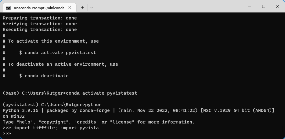
This will open up a Python shell. Type import tifffile; import pyvista and press Enter. If the packages are installed correctly, importing those packages shouldn’t give you any error messages, and your screen should look somewhat like the image below. If you did get any message, then something went wrong during installation, or you forgot to activate the pyvistatest environment.
You can now exit this Python shell by typing exit() (and pressing Enter).
Writing the visualization script
We’re going to start simple: we load an image file using tifffile, and then display it. Write the following Python code, and save it somewhere. (In this example, we’ll save it as my_pyvista_test.py.)
import tifffile
import pyvista

image_array = tifffile.imread(r"path/to/Dataset intestinal organoid proliferation/Microscopy images/nd799xy08/nd799xy08t099c1.tif")

print("Shape: ", image_array.shape)
print("Min value:", image_array.min())
print("Max value:", image_array.max())
Then change the path on line 4 to point to the image, and run the code from your Anaconda Prompt:
python path/to/my_pyvista_test.py
You can also run the script using Visual Studio Code, PyCharm or whatever, instead of using the command line. Interactive environments like Spyder or Jupyter likely won’t work out of the box, but you can work around that.
If the package tifffile and/or pyvista went missing, but they were successfully installed before, then you’re running the script from the wrong Anaconda environment. If everything went well, then you should see:
Shape: (30, 512, 512)
Min value: 0
Max value: 255
This indicates that the pixels in the image range from 0 to 255.
Next, we’re going to plot the image. Add the following code at the end of the file, and run the file again:
# Convert the array from ZYX (the TIFF file order) to XYZ (the Pyvista order)
image_array = image_array.swapaxes(0, 2)

# Create a PyVista grid that matchest the image dimensions
grid = pyvista.UniformGrid()
grid.dimensions = image_array.shape
grid.spacing = (0.32, 0.32, 2)  # This is the image resolution

# Create a smooth contour. Here, we show all pixels > 50, and hide those < 50
mesh = grid.contour([50], image_array.flatten(order="F"),
                    method='marching_cubes')
mesh.plot()
This results in the following image (at least, if you rotate the organoid a bit):
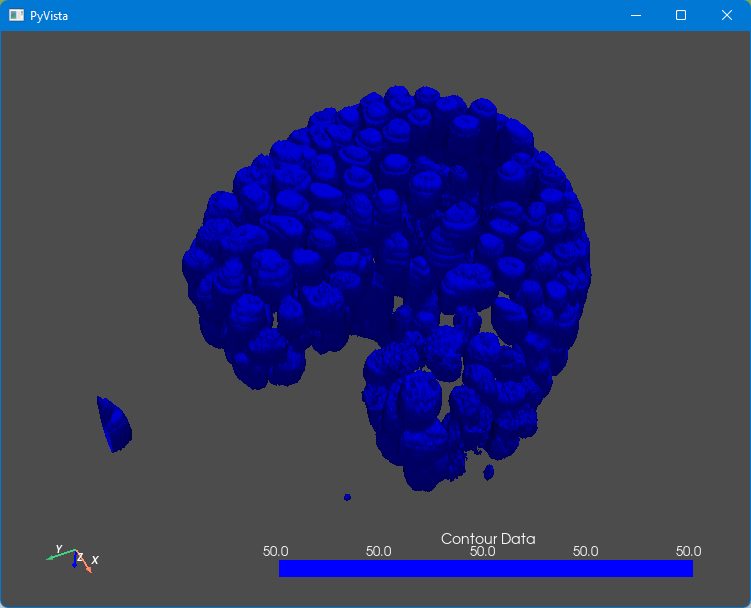
Ok, not bad, but it could look better. First, the image is still a bit blocky. We used the Marching Cubes method to estimate the contour between all pixels that are smaller than 50 and those that are larger than 50. We can smooth the contour a bit by adding the following line, just before the last line:
mesh = mesh.smooth(n_iter=1000)
Now rerun the script. (You’ll need to close the PyVista window first.) You can play with the number of iterations to obtain a result with more or less smoothing.
We will also change the last line a bit, to improve the coloring and lighting, and to hide that useless color bar:
mesh.plot(color="#ffffff", background="#0b0124", specular=0.1, show_scalar_bar=False)
(The colors used here are hexadecimal color codes.)
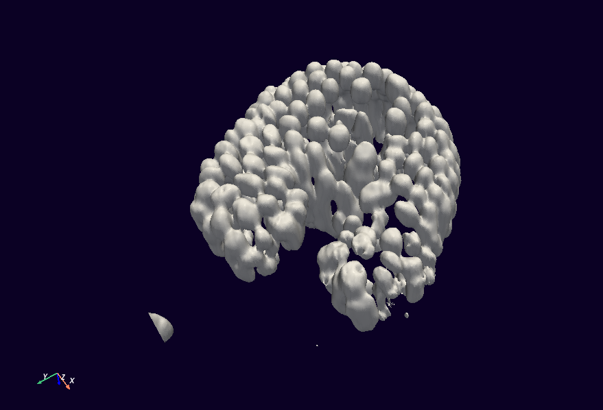
Job done!
Exploring from here
- Your image might be too noisy for this to work. If that’s the case, smooth it out first in ImageJ.
- You can save your organoid as a 3D object using
mesh.save("file.stl"). Recent versions of PowerPoint can directly load STL files, so you can surprise your audience with 3D object in PowerPoint. 😃