Using CellPose

In this tutorial, we’re going to install CellPose, which allows you to segment cells in images. It supports multiple kinds of images, from simple 2D light microscopy to 3D confocal stacks.

Terms and conditions

CellPose is free software developed by Carsen Stringer and Marius Pachitariu. If you use their software, you do need to acknowledge them, i.e. cite them if you’re writing a scientific paper. Some of their newer models are also only available for non-commercial use. See their Github page for more information

Installing everything

First, make sure you have installed Anaconda (see a tutorial here) and that you have downloaded the “Intestinal organoid crypts” dataset from the example data. Then, open the Anaconda Prompt and run the following command:

conda create --name cellposetest --channel conda-forge tifffile cellpose pyqt pyqtgraph

This will create an environment named “cellposetest” (feel free to choose a different name) with the packages tifffile, cellpose, pyqt and pyqtgraph, which it will all download from the conda-forge channel. The package tifffile allows us to read the TIFF files from the example dataset using Python, and the specifier --channel conda-forge is necessary because the CellPose package is not available from the default Anaconda download channel.

Note on PIP versus Anaconda: the official installation instructions of CellPose use an Anaconda environment too, but then proceed to install CellPose using PIP instead of Anaconda. I don’t really like mixing these two package managers, as it makes it harder to recreate your exact environment, and it can lead to having conflicting packages in the same environment. Since CellPose is also available as an Anaconda package nowadays, we can just install it from there and avoid PIP.

Trying the CellPose Graphical User Interface (GUI)

Now that everything is installed, we need to activate the CellPose environment. You need to do this each time you open the Anaconda Prompt.

conda activate cellposetest
cellpose

The first command activates the environment, the second starts up the CellPose GUI. You can drag an image in it from the example dataset, here we will use Dataset/Microscopy images/nd799xy08/nd799xy08t001c1.tif. The result then looks like this:

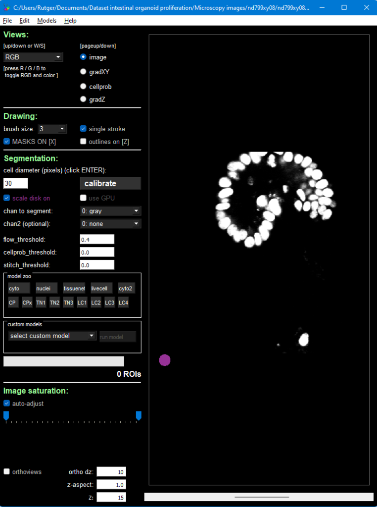
Press the big Calibrate button, which will estimate the size of your nuclei (or cells, if you’re using another image). The purple circle in the bottom left of the image should then roughly match your nucleus size. If it doesn’t, change its size manually using the text field on the left of the Calibrate button.

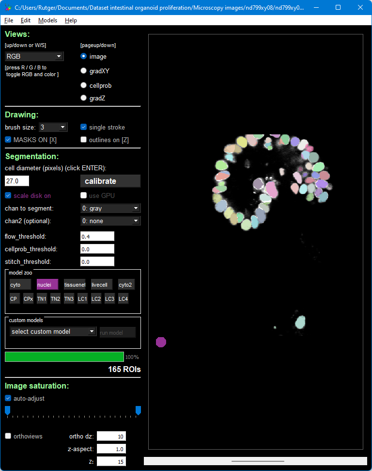
Then, press the “nuclei” button inside the area that’s titled “model zoo”. Because this is a 3D image, but the model is 2D, CellPose will repeatedly apply the model. After a few minutes, during which the program will hang (but the Anaconda Prompt should still show progress), you should see this result:

Running CellPose in a loop

This all works well for a single image, but as we’re on the Tracking Organoids website, you’ll likely want to run CellPose once for each image in a folder. For that, we’ll need to write a Python script.

Create a script with the following code:

import glob
import cellpose.models
import numpy
import tifffile

file_pattern = r"C:\Users\Rutger\Documents\Dataset intestinal organoid proliferation\Microscopy images\nd799xy08\nd799xy08t*c1.tif"  # Note the wildcard (*) in the file pattern
model = cellpose.models.Cellpose(gpu=False, model_type="nuclei")
channels = [0, 0]  # Channels, leave like this if you have grayscale images. See CellPose GUI for explanation.
anisotropy = 2 / 0.32  # Ratio Z-resolution / XY-resolution
diameter = 27  # Nucleus diameter in PX in XY

for file_path in glob.glob(file_pattern):
    image = tifffile.imread(file_path)
    print(f"Working on file {file_path}...")
    masks, flows, styles, estimated_diameter = model.eval(image, diameter=diameter, channels=channels, anisotropy=anisotropy, do_3D=True)

    output_file = file_path[:-4] + "_masks.tif"
    tifffile.imwrite(output_file, masks.astype(numpy.uint16), compression=tifffile.COMPRESSION.ADOBE_DEFLATE, compressionargs={"level": 9})

Then, modify line 6 to point to your dataset folder (from the example data). As you can see from the path in the script, we will use the organoid named nd799xy08.

Before we run the file, there are a few things to explain:

• First, we import some packages. glob is a Python built-in, and allows you to iterate over all files that match a pattern. This is used on line 12. numpy is used for arrays, cellpose for segmentation and tifffile for loading our example images.
• On line 7, we load the appropriate CellPose model, “nuclei” in our case.
• On line 8, we define the channels. Since we’re working with grayscale images, we simply leave these as [0, 0]. See the CellPose GUI for other possible numbers.
• On line 9, we define our “image anisitropy”, which is the ratio between the Z and XY resolution. In our case, our Z-resolution is 2 μm/px and our XY-resolution is 0.32 μm/px.
• On line 10, we use the pixel diameter of our nuclei. Here, we simply used the value that we got in the GUI after pressing Calibrate.
• The rest of the code is looping over all files that match the pattern. We load the images, apply CellPose to it, and then save the masks as a compressed 16-bit TIFF file. The output file name is output_file = file_path[:-4] + "_masks.tif", which means that “some/example.tif” becomes “some/example_masks.tif”.

After you’ve modified line 6, you can run the script from your Anaconda environment, and see how CellPose (slowly!) segments all your images. The images will be placed in the same folder as the input images, so Dataset intestinal organoid proliferation\Microscopy images\nd799xy08\ in this example.

That’s it! Congratulations, you now know how to segment your nuclei. You will have a so-called labeled image, where a pixel intensity of 0 represents the background, 1 represents the first nucleus, 2 the second, etc.

Opening a labeled image in ImageJ

ImageJ can nicely display these images, but it works a little bit clumsy. In this example, we will load the first image of time lapse nd799xy08.

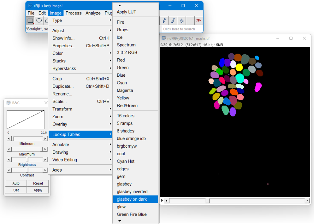
By default, ImageJ will set the minimum intensity to 0, and the maximum to 1. However, in our image the maximum intensity is 218, as there are 218 cells in this image. To change this, you first have to go to the last Z layer, so move the slider below the image to the last image. Then, in the ImageJ menu, select Image > Adjust > Brightness and Contrast, and drag the slider of the Maximum intensity all the way to the right. This will instruct ImageJ to scale the brightness from 0 to 218. You should now see an image with various shades of gray.

Next, we’re going to make the image a bit more colorful. Use Image > Lookup Tables > glasbey on dark. If everything worked well, then you should see this:

Speeding things up using a graphics card (GPU)

First, you need to change one line in the above script: on line 7, change gpu=False to gpu=True.

Second, we need to install the GPU-enabled version of Pytorch into our Anaconda environment. So open up your Anaconda Prompt and activate the CellPose environment, and install the CUDA-enabled Anaconda version of PyTorch. Instructions for that are available on this webpage. There is one difference: you can leave out torchvision and torchaudio from the resulting command, since CellPose doesn’t use those packages.

For me, the command I got was: (after leaving out torchvision and torchaudio)

conda install pytorch pytorch-cuda=11.6 --channel pytorch --channel nvidia

Note about a difference with the official CellPose instructions: in the official installation instructions of CellPose, they say to remove the PIP version of PyTorch first using pip uninstall torch. Since we installed everything through Anaconda, we don’t need to manually resolve this package conflict.

Hopefully everything works out using these instructions. Although running computations on a GPU is becoming easier every year, the installation can still be difficult sometimes.

Further information

• CellPose 2.0 introduced more models, as well as making it easier to train your own model. See this section for more information.
• You can also play around with your images (like changing the brightness and contrast) to make them work better with an existing model of CellPose.